Listen to this audio overview to quickly understand Event-Related Potentials (ERPs) and their importance in neuroscience research.
An event-related potential (ERP) is a measured brain response that is the direct result of a specific sensory, cognitive, or motor event. Essentially, it is the electrical activity in the brain that occurs in reaction to an external stimulus or an internal cognitive process, such as recognizing a word or hearing a sound. ERPs are derived from electroencephalography (EEG) by averaging the brain's electrical response to repeated presentations of a stimulus, helping researchers identify how the brain processes these events over time.
ERP signals consist of distinct deflections or peaks, which are traditionally named based on their order and polarity (positive or negative) as they occur in the timeline following the stimulus. For example, the "P300" component is a prominent positive deflection that typically occurs around 300 milliseconds after the stimulus. Peaks and components refer to identifiable features of the ERP waveform that are associated with different stages of information processing.
Each component provides information about how different cognitive processes unfold over time, allowing researchers to make inferences about brain function.


The averaging and processing of ERPs provide a valuable tool for understanding the timing and stages of cognitive and perceptual processes in the brain, making them particularly useful in fields such as psychology, neuroscience, and clinical diagnostics.
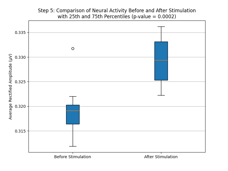
Below is an example of Python code that demonstrates how to process EEG data to obtain an ERP. This code uses simulated EEG data to illustrate key steps such as filtering, epoching, and averaging. Additionally, the code includes visualization steps that help in understanding the different stages of ERP analysis, from raw EEG data to the averaged ERP waveform.
The Python code walks through the following steps:
import numpy as np
import matplotlib.pyplot as plt
from scipy.signal import butter, filtfilt
from scipy.stats import ttest_rel
import os

# Simulated EEG Data Parameters
np.random.seed(42)
sampling_rate = 1000  # in Hz
duration = 11  # in seconds (extended to ensure space for response after the last stimulus)
n_samples = sampling_rate * duration

# Define Stimulus Onsets
stimulus_interval = 1  # in seconds
stimulus_onsets = [i * stimulus_interval for i in range(1, 11)]  # stimulus at 1.0s, 2.0s, 3.0s, ..., 10.0s

# Simulate EEG Data (with noise)
time = np.linspace(0, duration, n_samples, endpoint=False)
eeg_data = 0.5 * np.sin(2 * np.pi * 10 * time) + 0.2 * np.sin(2 * np.pi * 20 * time) + 0.1 * np.random.randn(n_samples)  # 10 Hz and 20 Hz signals with noise

# Add Consistent Simulated Response to Stimulus with Varying Amplitude
response_duration = int(0.1 * sampling_rate)  # 100 ms post-stimulus response
for onset in stimulus_onsets:
    response_amplitude = 0.3 + 0.05 * np.random.randn()  # Add noise to the amplitude of the response
    response = response_amplitude * np.exp(-np.linspace(0, 1, response_duration)) * np.sin(2 * np.pi * 15 * np.linspace(0, 0.1, response_duration, endpoint=False))
    start_idx = int(onset * sampling_rate)
    end_idx = start_idx + response_duration
    if end_idx <= len(eeg_data):
        eeg_data[start_idx:end_idx] += response  # Ensure the complete response is added

# Define Bandpass Filter for Filtering EEG Data
def butter_bandpass(lowcut, highcut, fs, order=4):
    nyquist = 0.5 * fs
    low = lowcut / nyquist
    high = highcut / nyquist
    b, a = butter(order, [low, high], btype='band')
    return b, a

def bandpass_filter(data, lowcut, highcut, fs, order=4):
    b, a = butter_bandpass(lowcut, highcut, fs, order=order)
    y = filtfilt(b, a, data)
    return y

# Filter the EEG Data
filtered_eeg = bandpass_filter(eeg_data, lowcut=1, highcut=30, fs=sampling_rate)

# Segment the EEG Data (Epoching)
epochs = []
epoch_window = int(1.0 * sampling_rate)  # 500 ms before and after stimulus
for onset in stimulus_onsets:
    start_idx = int((onset - 0.5) * sampling_rate)  # 500 ms before onset
    end_idx = int((onset + 0.5) * sampling_rate)  # 500 ms after onset
    if start_idx >= 0 and end_idx <= len(filtered_eeg):
        epochs.append(filtered_eeg[start_idx:end_idx])

# Average the Epochs to Obtain ERP
if len(epochs) > 0:
    erp = np.mean(epochs, axis=0)
else:
    erp = np.zeros(epoch_window)

# Create directory for saving figures
output_dir = "ERPs/static"
os.makedirs(output_dir, exist_ok=True)

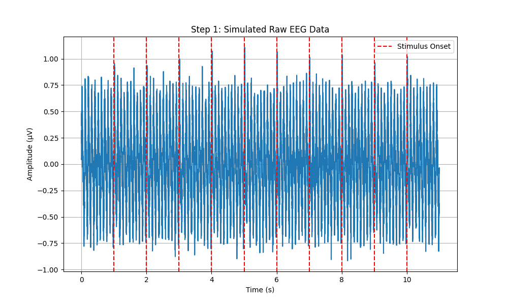
# Plot Raw EEG Data with Stimulus Onsets
plt.figure(figsize=(10, 6))
plt.plot(time, eeg_data)
for onset in stimulus_onsets:
    plt.axvline(x=onset, color='r', linestyle='--', label='Stimulus Onset' if onset == stimulus_onsets[0] else None)
plt.xlabel('Time (s)')
plt.ylabel('Amplitude (µV)')
plt.title('Step 1: Simulated Raw EEG Data')
plt.legend()
plt.grid(True)
plt.savefig(os.path.join(output_dir, 'step1_raw_eeg.png'))
plt.close()

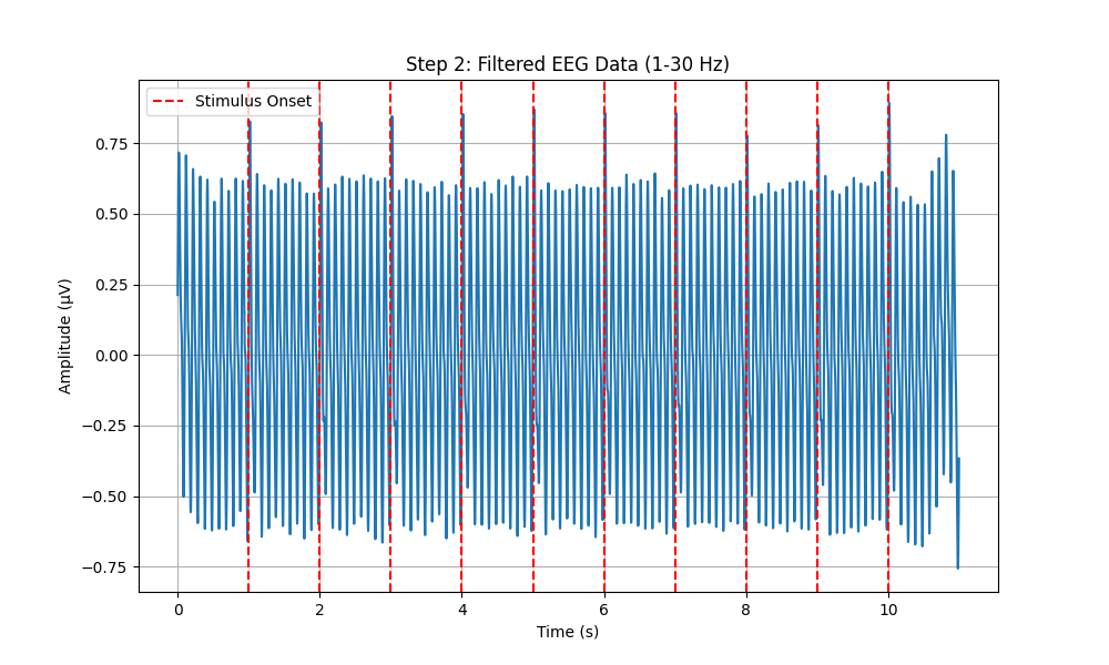
# Plot Filtered EEG Data with Stimulus Onsets
plt.figure(figsize=(10, 6))
plt.plot(time, filtered_eeg)
for onset in stimulus_onsets:
    plt.axvline(x=onset, color='r', linestyle='--', label='Stimulus Onset' if onset == stimulus_onsets[0] else None)
plt.xlabel('Time (s)')
plt.ylabel('Amplitude (µV)')
plt.title('Step 2: Filtered EEG Data (1-30 Hz)')
plt.legend()
plt.grid(True)
plt.savefig(os.path.join(output_dir, 'step2_filtered_eeg.png'))
plt.close()

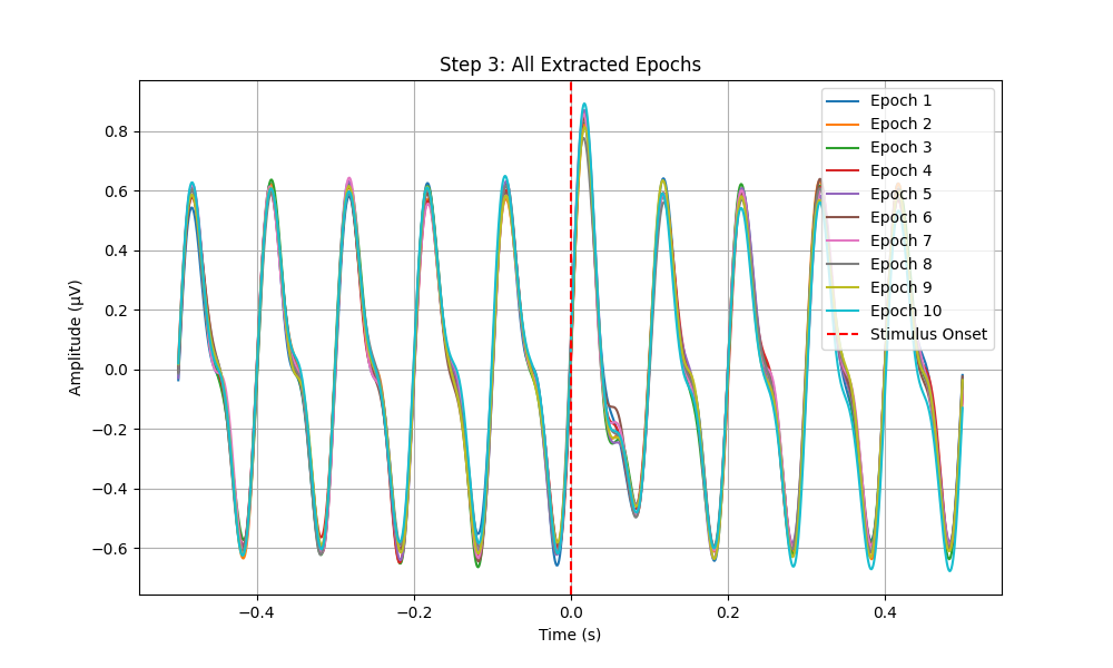
# Plot All Epochs
plt.figure(figsize=(10, 6))
for i, epoch in enumerate(epochs):
    plt.plot(np.linspace(-0.5, 0.5, len(epoch), endpoint=False), epoch, label=f'Epoch {i+1}')
plt.xlabel('Time (s)')
plt.ylabel('Amplitude (µV)')
plt.title('Step 3: All Extracted Epochs')
plt.axvline(x=0, color='r', linestyle='--', label='Stimulus Onset')
plt.legend()
plt.grid(True)
plt.savefig(os.path.join(output_dir, 'step3_all_epochs.png'))
plt.close()

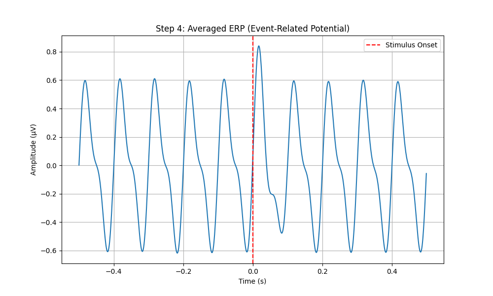
# Plot the ERP
plt.figure(figsize=(10, 6))
plt.plot(np.linspace(-0.5, 0.5, len(erp), endpoint=False), erp)
plt.xlabel('Time (s)')
plt.ylabel('Amplitude (µV)')
plt.title('Step 4: Averaged ERP (Event-Related Potential)')
plt.axvline(x=0, color='r', linestyle='--', label='Stimulus Onset')
plt.legend()
plt.grid(True)
plt.savefig(os.path.join(output_dir, 'step4_averaged_erp.png'))
plt.close()

# Plot Boxplot to Compare Neural Activity Before and After Stimulation
pre_stimulus_values = [np.mean(np.abs(epoch[:int(epoch_window / 2)])) for epoch in epochs]  # Mean of absolute values before stimulus (first 500 ms)
post_stimulus_values = [np.mean(np.abs(epoch[int(epoch_window / 2):])) for epoch in epochs]  # Mean of absolute values after stimulus (last 500 ms)

# Perform a paired t-test to determine significance
stat, p_value = ttest_rel(pre_stimulus_values, post_stimulus_values)

plt.figure(figsize=(8, 6))
plt.boxplot([pre_stimulus_values, post_stimulus_values], labels=['Before Stimulation', 'After Stimulation'], patch_artist=True)
plt.ylabel('Average Rectified Amplitude (µV)')
plt.title(f'Step 5: Comparison of Neural Activity Before and After Stimulation\nwith 25th and 75th Percentiles (p-value = {p_value:.4f})')
plt.grid(axis='y')
plt.savefig(os.path.join(output_dir, 'step5_comparison_boxplot.png'))
plt.close()